Animating LiDAR point clouds in R
Recently I gave a brief presentation at CUGOS about some LiDAR animations I’ve been working on. There was a fair amount of ooh and aah (if I do say so myself), so this post is a brief how-to of how to animate LiDAR data in R. As an example, here is an animation of downwelling radiation in a forest canopy during a typical day in August.
I started working on this because I was taking a LiDAR cloud, which is already 3-dimensional, and adding a temporal dimension with data from the flux tower in Wind River Experimental Forest. Visualizing 4-dimensions statically is really hard, and animations are really pretty anyway.
I’m going to assume that you have basic knowledge of working with LiDAR data in R. If not, I highly recommend the lidR book and this tutorial from NSF NEON. We aren’t going to use any of the processing features in lidR, so if you know how to plot a cloud with it you are good to go. Also, this approach only works well with small clips of airborne LiDAR. If you have a huge dataset, rgl will really struggle.
Setup
There are three key packages: lidR, rgl, and rglplus. lidR is the most popular R package for reading and manipulating LiDAR data, while rgl and rglplus provide 3D visualization utilities.
We generate animations with the function rglplus::rgl.makemovie. This function calls ffmpeg under the hood to convert a series of image files into an MP4 video. You will need to have ffmpeg installed and accessible from the RStudio terminal for this to work. If you don’t have that for some reason, rgl.makemovie will generate a directory of image files for each frame of the animation. You can then encode all of those into a video with the tool of your choice.
With all that said, let’s build the structure of our first animation.
library(lidR)
library(rgl)
library(rglplus)

# Toy data included with lidR
LASfile <- system.file("extdata", "MixedConifer.laz", package="lidR")
las <- readLAS(LASfile)
The way we generate animations is with rglplus::rgl.makemovie. This function works by effectively taking a screenshot of the active rgl scene, and then concatenating all of those together in an MP4 video using ffmpeg. Fortunately for us, lidR::plot uses rgl as its backend, so we can easily pair those two together. The most important argument to rgl.makemovie is frame. frame is a function of one argument that updates the current rgl context before the next frame of the animation is captured.
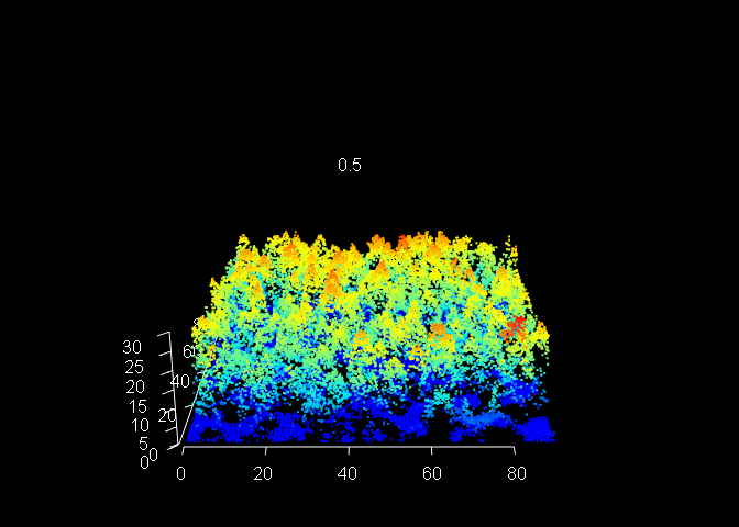
To start with, we are just going to plot the point cloud and add some text indicating the current frame time. Call the function and you should see the cloud with some text, like so.
my_frame_func <- function(t) {
  close3d()            # Close the current scene if one exists
  plot(las, axis=TRUE) # Plot the point cloud
  display_t <- as.character(round(t, 2))
  text3d(40, 40, 60, display_t, color="white") # add text at the point (40, 40, 60)
}
my_frame_func(0.5)
Now let’s call this function with rgl.makemovie.
anim_time <- 1
fps <- 30
out_dir <- tempdir()

rgl.makemovie(frame=my_frame_func, tmin=0, tmax=anim_time, fps=fps,
              nframes = anim_time * fps,
              output.path=out_dir,
              output.filename="my_movie1.mp4",
              quiet=FALSE)
You should see a bunch of output, and a series of rgl windows opening and closing quickly. In the above, I’m writing the output to a temporary directory. If you open that directory, you should see a file called my_movie.mp4. Open the video, and you should see a simple render of your point cloud and some white text that goes from 0 to 1. Now let’s build from this.
3D visualization parameters
rgl gives us several ways to play with the camera and window size that are exposed through the function par3d. This function returns a named list with all the grahpics settings of the current scene. Plot up the point cloud and then call this function.
plot(las, axis=TRUE)
par3d()
## $antialias
## [1] 8
##
## $FOV
## [1] 30
##
## $ignoreExtent
## [1] FALSE
##
## $listeners
## [1] 472
##
## $mouseMode
##        none        left       right      middle       wheel
##      "none" "trackball"      "user"       "fov"      "pull"
##
## $observer
## [1]   0.000   0.000 253.424
##
## $modelMatrix
##      [,1]       [,2]      [,3]       [,4]
## [1,]    1  0.0000000 0.0000000  -44.99500
## [2,]    0  0.3420202 0.9396926  -30.44178
## [3,]    0 -0.9396926 0.3420202 -216.66910
## [4,]    0  0.0000000 0.0000000    1.00000
##
## $projMatrix
##          [,1]     [,2]      [,3]      [,4]
## [1,] 3.732051 0.000000  0.000000    0.0000
## [2,] 0.000000 3.732051  0.000000    0.0000
## [3,] 0.000000 0.000000 -3.863703 -913.5641
## [4,] 0.000000 0.000000 -1.000000    0.0000
##
## $skipRedraw
## [1] FALSE
##
## $userMatrix
##      [,1]       [,2]      [,3] [,4]
## [1,]    1  0.0000000 0.0000000    0
## [2,]    0  0.3420201 0.9396926    0
## [3,]    0 -0.9396926 0.3420201    0
## [4,]    0  0.0000000 0.0000000    1
##
## $userProjection
##      [,1] [,2] [,3] [,4]
## [1,]    1    0    0    0
## [2,]    0    1    0    0
## [3,]    0    0    1    0
## [4,]    0    0    0    1
##
## $scale
## [1] 1 1 1
##
## $viewport
##      x      y  width height
##      0      0    256    256
##
## $zoom
## [1] 1
##
## $bbox
## [1]  0.00 89.99  0.00 89.90  0.00 32.07
##
## $windowRect
## [1] 138 161 394 417
##
## $family
## [1] "sans"
##
## $font
## [1] 1
##
## $cex
## [1] 1
##
## $useFreeType
## [1] FALSE
##
## $fontname
## [1] "TT Arial"
##
## $maxClipPlanes
## [1] 8
##
## $glVersion
## [1] 4.6
##
## $activeSubscene
## [1] 0
There’s a lot going on here, most of which we don’t really care about. Reading the documentation is a good place to start understanding what all this means, but it is also helpful to play with the cloud and then call par3d again. Resize the window, then viewport and windowRect change. Click and drag the cloud, then userMatrix and modelMatrix change. There are 4 parameters we care about: userMatrix, userProjection, windowRect, and scale.
This gives us a way to set up a window size and view angle and then apply it to an animation. Try changing the scene around, then save the parameters in a list. We can then supply this to par3d in our frame function. One important detail is that the window size must be divisible by 2 for the conversion to MP4 to work.
# After moving the cloud around...
mypar <- par3d()[c("userMatrix", "userProjection",
                   "windowRect", "scale")]

# Make sure the window size is divisible by 2
mypar$windowRect <- round(mypar$windowRect/2) * 2

my_frame_func2 <- function(t) {
  # Same as before...
  my_frame_func(t)
  # Except now we set the new view parameters
  par3d(mypar)
}

rgl.makemovie(frame=my_frame_func2, tmin=0, tmax=anim_time, fps=fps,
              nframes = anim_time * fps,
              output.path=out_dir,
              output.filename="my_movie2.mp4",
              quiet=FALSE)
Now you should get a new animation with the camera and window size adjusted like before. Next, we will learn how to manipulate the point cloud within the scene.
Rotating the cloud
If we want the point cloud to move within our scene, we have two options: move the camera, or move the point cloud. In my experience I find moving the point cloud easier. But, you could also accomplish this by modifying userMatrix and observer with par3d.
At its core, LiDAR data is just a matrix of points in 3D space. The lidR package lets us access that data through the $data slot. To rotate points in 3D space, we turn to rotation matrices. This can be a little tricky, so let’s start by just rotating our existing point cloud.
Rotation matrices will spin points around the origin (0, 0, 0). But, if we check the data in our point cloud, we find that the points are far from the origin.
las
## class        : LAS (v1.2 format 1)
## memory       : 2.2 Mb
## extent       : 481260, 481350, 3812921, 3813011 (xmin, xmax, ymin, ymax)
## coord. ref.  : NAD83 / UTM zone 12N
## area         : 8072 m²
## points       : 37.7 thousand points
## density      : 4.67 points/m²
## density      : 4.67 pulses/m²
You can still do the rotation without accounting for the offset, but the result will be way off in space. So, really we have three steps.
- Center the original data at the origin
- Apply the rotation
- Re-offset the rotated data at the original position (if needed)
Fortunately this is pretty easy since we can get the appropriate offset with the mean of each coordinate.
offset <- c(
  mean(las$X),
  mean(las$Y),
  mean(las$Z)
)

# Only grab the XYZ coordinates
las_data <- las@data[, 1:3]
# Sweep subtracts a constant from each column
# See https://stackoverflow.com/questions/24520720/subtract-a-constant-vector-from-each-row-in-a-matrix-in-r
las_data_center <- sweep(las_data, 2, offset, FUN="-")

# Check that it worked - ranges are centered on zero
apply(las_data_center, 2, range)
##              X         Y         Z
## [1,] -45.19922 -45.23283 -12.01463
## [2,]  44.79078  44.66717  20.05537
With our data centered, we can now rotate it without messing up the coordinate space. First we make the rotation matrix. For more complex movements, you can also use rgl::rotationMatrix.
# ~45 degrees in radians
theta <- 0.785
# Manually create the matrix
rot_mtx_y45 <- matrix(
  c(
     cos(theta),  0, sin(theta),
              0,  1,          0,
    -sin(theta),  0, cos(theta)
  ),
  nrow=3, ncol=3
)
Then we apply the matrix to our centered data.
# Make sure to use the matrix multiplication operator!
# t() is the transpose function, it ensures the matrix dimensions
# remain how we want them.
las_data_center_rotate <- t(rot_mtx_y45 %*% t(las_data_center))
Next we reapply the offset so the rotated cloud is near the old one. You can ignore this step if you don’t care about having similar coordinates to the original, it won’t affect the animation result.
# Do the reverse of the sweep call from before
las_data_rotate <- sweep(las_data_center_rotate, 2, offset, FUN="+")
# Check that it worked again - ranges are similar to the original cloud.
apply(las_data_rotate, 2, range)
##          [,1]    [,2]      [,3]
## [1,] 481265.5 3812921 -28.41818
## [2,] 481345.3 3813011  52.62642
Finally, we rebuild the LAS object so we can plot it. Modifying the data slot directly like this can invalidate the internal LAS specification, preventing you from saving out the rotated data. But if you only care about animating then it’s whatever. If you know of a less hacky way, let me know :)
las_rotate <- las
las_rotate@data[, 1] <- las_data_rotate[, 1]
las_rotate@data[, 2] <- las_data_rotate[, 2]
las_rotate@data[, 3] <- las_data_rotate[, 3]

plot(las_rotate, axis=TRUE)
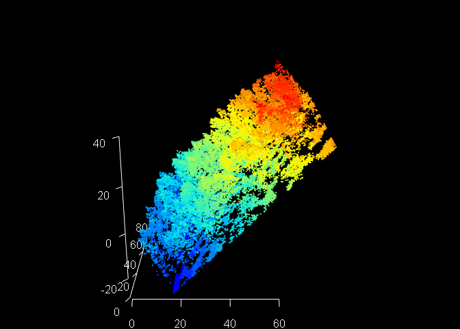
And there you go, a point cloud on a slant. You may be asking yourself why on Earth you would ever need this. One example is modeling how light moves through a canopy. Sunlight almost never hits a forest canopy at nadir, and accounting for solar angle can be important in early morning or high-latitude environments.
Bring it all together
Now let’s animate a spinning cloud. First, let’s functionalize some code.
rot_matrix_y <- function(theta) {
  # Make a rotation matrix about the y axis
  matrix(
    c(
       cos(theta),  0, sin(theta),
                0,  1,          0,
      -sin(theta),  0, cos(theta)
    ),
    nrow=3, ncol=3
  )
}

rotate_las <- function(las, rot_mtx, do_offset=TRUE) {
  if (do_offset) {
    offset <- c(
      mean(las$X),
      mean(las$Y),
      mean(las$Z)
    )
  } else {
    offset <- c(0, 0, 0)
  }

  las_data_center <- sweep(las@data[, 1:3], 2, offset, FUN="-")
  las_data_center_rotate <- t(rot_mtx %*% t(las_data_center))
  las_data_rotate <- sweep(las_data_center_rotate, 2, offset, FUN="+")

  new_las <- las
  new_las@data[, 1] <- las_data_rotate[, 1]
  new_las@data[, 2] <- las_data_rotate[, 2]
  new_las@data[, 3] <- las_data_rotate[, 3]

  new_las
}
Now we modify the frame function to rotate the cloud at an angle dependent on the animation time.
my_frame_func3 <- function(t) {
  close3d()
  # Use the animation time as the rotation angle
  theta <- t
  # Rotate the cloud
  rot_mtx <- rot_matrix_y(theta)
  las_rotate <- rotate_las(las, rot_mtx)
  # Plot everything else as before
  plot(las_rotate, axis=TRUE)
  display_t <- as.character(round(t, 2))
  text3d(40, 40, 60, display_t, color="white")
}
And we should now get a video of a spinning point cloud. I’m changing the frame time and fps so it doesn’t take as long to animate.
anim_time <- 6.28 # get a full rotation
fps <- 15
rgl.makemovie(frame=my_frame_func3, tmin=0, tmax=anim_time, fps=fps,
              nframes = anim_time * fps,
              output.path=out_dir,
              output.filename="my_movie3.mp4",
              quiet=FALSE)
And there you have it. This only scratches the surface of what is feasible with lidR and rgl. We could just as easily compute something about the point cloud in each frame and modify the color ramp to represent that (I did exactly that in the example embedded at the start of this post) Although this approach is fairly hacky, there are not many open-source tools that let you build animations with LiDAR. The next best option, especially for large datasets, would probably be the animation plugin in CloudCompare (example here). However, that approach is not programmatic, does not allow editing the point color, and requires you to set key frames manually.